Segmenting Twitter Followers using PCA and Clustering

The data was collected as part of a study using followers of the Twitter account of a huge consumer brand. The brand wants to understand its twitter audience better to fine-tune its Twitter posts. To achieve this, they collected every twitter post of a sample of its followers and each post was examined by Amazon’s Mechanical Turk and was categorized into different interest areas.

The task is to analyze this data and identify any interesting market segments among the social media followers.

The Dataset

Let’s look at the data.

head(social_m_raw,5)

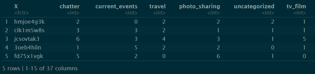
Each row in the data represents a user and the column represents the interests of the user. The entries are the number of posts by a user that fell into the given category. For example, the first user has posted two times about travel and once about tv or film. Similarly, the third user has posted six times about chatter, three times about current events and so on. I hope you get the idea!

There are 36 broad categories that a user can post about. After examining the 36 columns, I suspect correlation among these variables. Let’s look at the correlation plot.

Correlation plot

cormat <- round(cor(social_m_raw[,2:37]), 2)
corrplot(cormat, method=”circle”)

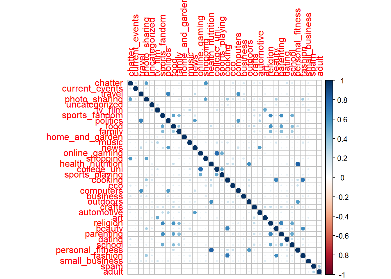
A lot of variables are correlated with each other. For instance, personal fitness and healthy nutrition are highly correlated. Also, online gaming and college university variables have a high correlation. Let’s use PCA to reduce the dimensions to create a fewer number of uncorrelated variables.

Why PCA?

Principal Component Analysis is a type of dimension reduction. PCA creates uncorrelated principal components from the original correlated variables such that the principal components are the linear combination of the original variables. The principal components are ranked in the order the proportion of variance explained. For instance, the first principal component explains the highest proportion of variation among all other principal components.

Nice visualization of PCA

pca_sm = prcomp(social_m_raw[,2:32], scale=TRUE, center = TRUE)
pca_var <- pca_sm$sdev ^ 2
pca_var1 <- pca_var / sum(pca_var)
#Cumulative sum of variation explained
plot(cumsum(pca_var1),xlab =“Principal Component”,ylab =“Fraction of variance explained”)
abline(v = 16, h=0.8, col=’red’)

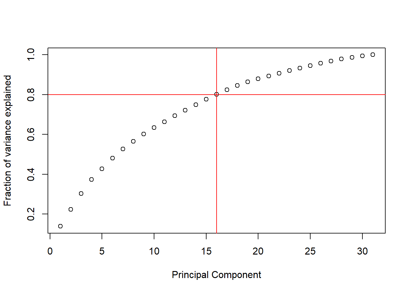
The plot above shows the cumulative sum of the proportion of variance explained for every additional principal component. We can see from PCA results that 80% of the variation is explained by the first sixteen principal components. But how do we pick the correct number of principal components?

According to the Kaiser criterion, we should drop all the principal components with eigenvalues less than 1.0. Read about it here: Kaiser Criterion. There are a lot of debates on how to pick the optimum number of principal components. Let’s use the Kaiser criterion here.

summary(pca_sm)

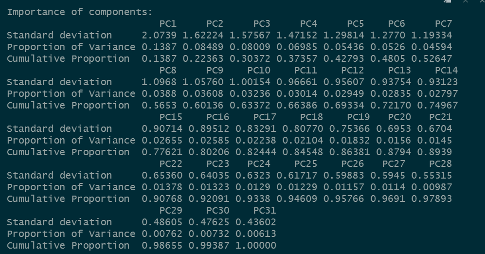
We can see that the first ten principal components explain 63.3% of the variance and have an eigenvalue greater than one. One more important concept we should understand is loadings. Loadings explain the relationship of the principal components with the original variable. Let’s use the varimax rotation to explain the loadings. There are a bunch of rotation methods available.

varimax(pca_sm$rotation[, 1:11])$loadings

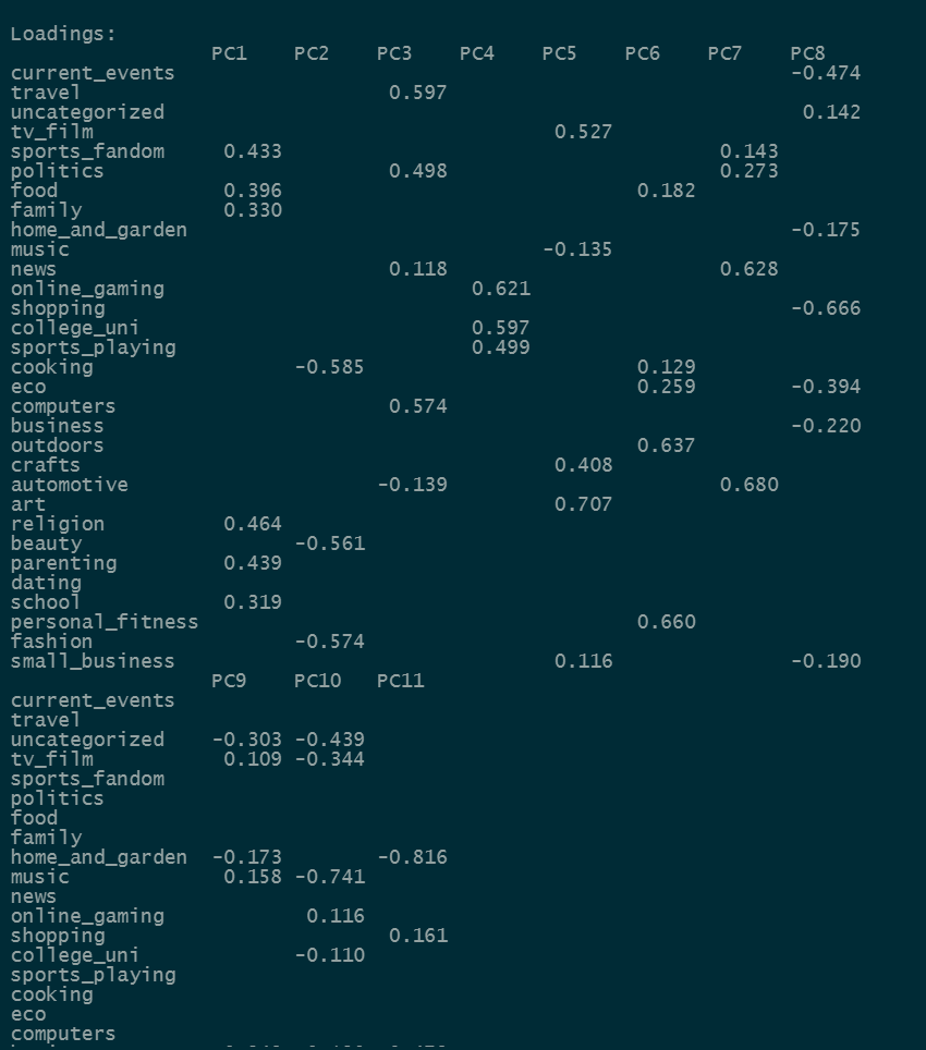
The first principal component is a linear combination of sports_fandom, food, family, religion, parenting and school variables, and their weights are given in the above result. So we can say

PC1 = 0.433 x sports_fandom + 0.396 x food + 0.330 x family + 0.464 x religion + 0.439 x parenting + 0.319 x school

Similarly, you can derive the other principal components.

Now let’s use the new data in the principal component space to run clustering.

scores = pca_sm$x
pc_data <- as.data.frame(scores[,1:10])
X <- pc_data

K-means clustering

Let’s use the kmeans++ initialization this time.

library(LICORS)
# Determine number of clusters
#Elbow Method for finding the optimal number of clusters
set.seed(123)
# Compute and plot wss for k = 2 to k = 15.
k.max <- 15
data <- X 
wss <- sapply(1:k.max, 
 function(k){kmeanspp(data, k, nstart=10,iter.max = 10 )$tot.withinss})
wss
plot(1:k.max, wss, type=”b”, pch = 19, frame = FALSE, 
 xlab=”Number of clusters K”,
 ylab=”Total within-clusters sum of squares”)

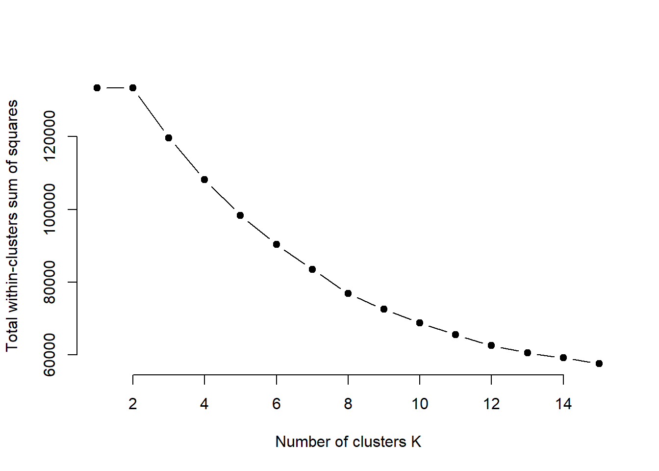
It is hard to decide the K here as we do not see an obvious elbow point. How do we pick the ideal number of clusters? The answer is ‘it depends!’. Always pick a k after which either the total within sum of squares is almost constant or a k that satisfies your requirement. Let’s pick 5 clusters since it is easier to understand five segments (I ran multiple iterations of clustering before I picked 5)

# Run k-means with 5 clusters and 15 starts
clust1 = kmeanspp(X, 5, nstart=15)
social_clust1 <- cbind(social_m, clust1$cluster)
plotcluster(social_m[,2:32], clust1$cluster)

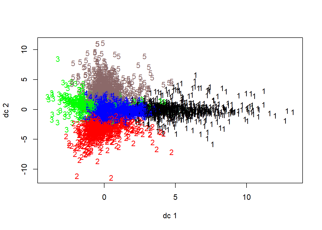
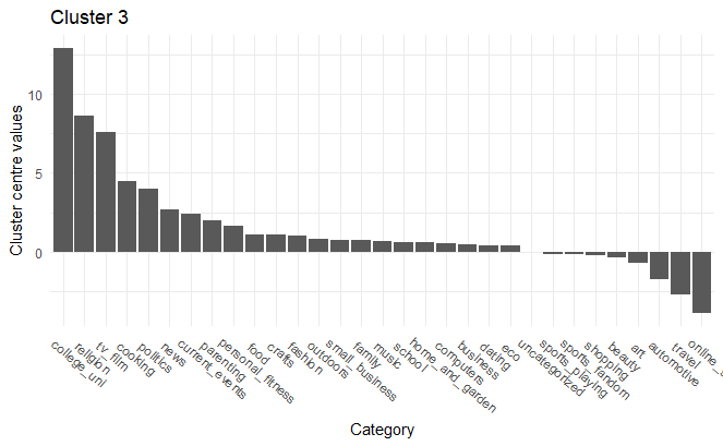
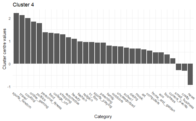
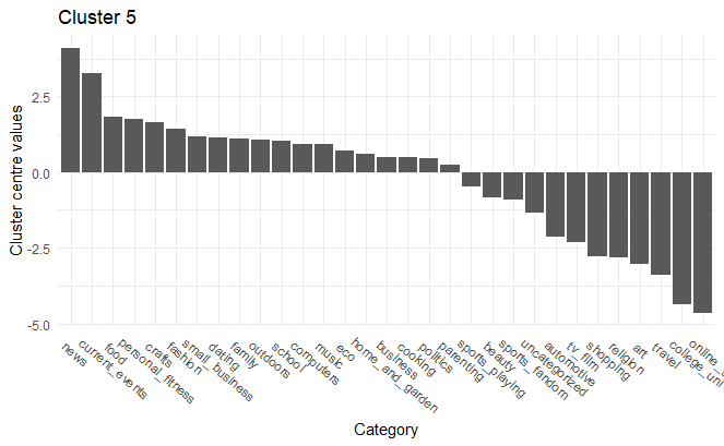
As we can see the data points are reasonably seperated with K = 5. Let’s use the cluster centers values to identify the differentiating characteristics of each cluster. Plot the cluster center value for each of the original column values to segment the customers and arrive at the final insights.

Results

Market segments identified:

1. Online gaming, News, Travel

2. Shopping, Art, News

3. College/university, Religion, TV & film

4. Sports Fandom, Travel, Cooking

5. News, Current Events and Food

Market segments identified:

1. Online gaming, News, Travel

2. Shopping, Art, News

3. College/university, Religion, TV & film

4. Sports Fandom, Travel, Cooking

5. News, Current Events and Food

Conclusion

Based on the K-Means clustering, we can identify distinct market segments that the firm can potentially leverage to design specific marketing campaigns. For example, Cluster 1— “ Online gaming, News, Travel” and Cluster 3— “College/university, Religion, TV & film” differ vastly in terms of interests. Cluster 3 consists mainly of religious college students who love TV and film shows. Furthermore, the individuals in this cluster are not inclined towards online-gaming or travel. However, cluster 1 individuals love online-gaming and traveling and do not like dating or art. Cluster 2 consists of individuals inclined towards shopping and art. People in cluster 4 are interested in Sports Fandom, Travel, Cooking while they are not so interested in current events, crafts or small business topics. In contrast, cluster 5 consists of people who have a penchant for news and current events. The cluster 5 individuals are also interested in personal fitness and fashion.

The brand can use the identified market segments to fine-tune its social media posts and improve the customer experience.